Highlighting alternate rows makes the spreadsheet more readable.
In this article, we will share a simple technique to highlight alternate rows in Excel.

How to Highlight Every Other Row in MS Excel
- Using a custom formula to highlight every other row
Method 1: Conditional Formatting through A Formula
To highlight every other row, we’ll need to create a custom conditional formatting rule. This will involve inputting out a formula and setting the custom format for your cells.
Step 1: Open up your Microsoft Excel file.

Step 2: Select the cells that you want the conditional formatting to apply to.
With your Excel file open, go ahead and select the cells where you want every other row to be highlighted.
Simply left-click and drag your mouse across the rows and columns to create a selection.
You can also do this by clicking on any row and highlighting the rest by pressing the Shift + Arrow keys.

Step 3: Go to the Conditional Formatting tab and select ‘More Rules.’
From there, under the Home tab, click on the Conditional Formatting button near the center and top part of Microsoft Excel.
Now, hover over Highlight Cells Rules and from the drop-down menu, click on More Rules…

Step 4: Select the custom formula Rule Type and input the formula.
A window, New Formatting Rule, should open up on your screen.
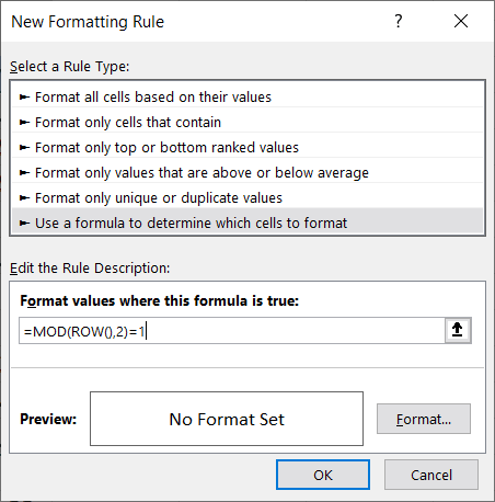
Under Rule Type:, select Use a formula to determine which cells to format. After that, you should be able to input the formula that will highlight every other row in your Excel file.
Under Format values where this formula is true:, type in:
=MOD(ROW(),2)=1
Where:
= MOD() – an Excel function that returns the remainder of two numbers after being divided
= ROW() – an Excel function that returns the number of the row specified in the formula. In this case, ROW() is empty, so it returns the row number where ROW() is present.
2 – refers to the divisor that is used in the MOD() function.
= 1 – the operation that determines whether a row is highlighted or skipped. If the remainder is equal to 1 (=1), then that row will be highlighted.
The window should look like the image below:
Step 5: Highlighting the cells with the color of your choice.
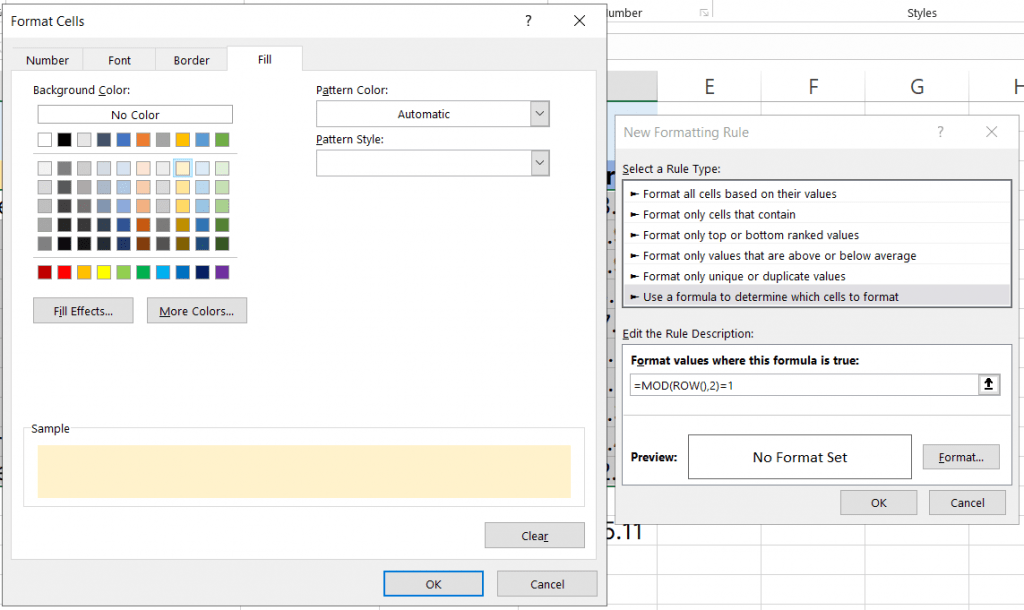
Before you click on OK, you have to figure out the format of the cells you’ve been highlighting. Simply click on Format… and you should be brought to a new window, with multiple tabs.
From there, go to the Fill tab and click on a color of your choice.
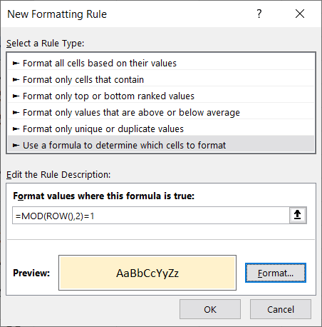
Once you’ve picked out a color, click on OK and you should see by the Preview: box an example of the format you’ve chosen.
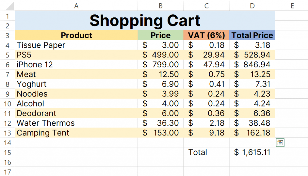
From there, simply click on OK and your cells should now be highlighted at every other row!
Editing or Deleting Conditional Formatting Rules
Once you’ve formatted and finalized the conditional formatting rules, finding them again can be confusing. In this method, we’ll show you where you can find all the active conditional formatting rules on your Excel sheet, as well as teach you how to edit them.
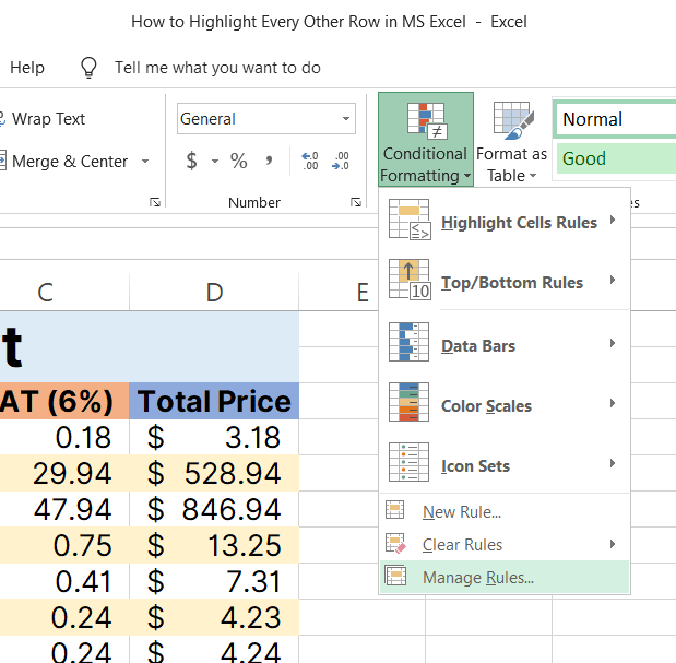
Step 1: With your Excel file open, navigate to Manage Rules.
Click on Conditional Formatting. You’ll find this at the top and center portion of Microsoft Excel. From there, click on Manage Rules.
Step 2: Show formatting rules for this worksheet.
A window should pop up on your screen. From there, open up the drop-down menu beside the Show formatting rules for: section and select This Worksheet.
That should display all active formatting rules on your worksheet.

Step 3: Editing Or Deleting the Conditional Format rules.
From the window on your screen, look for the formatting rule you want to edit and highlight it by selecting the rule.
If you want to delete the selected rule, simply click on Delete Rule near the top left corner of the window.

Otherwise, simply double-click the rule to edit the formatting rule. You can also select the rule and click on Edit Rule for the same effect.

Simply click on the Format button to change the format or select a new rule type if you want to redo the rule.
Conclusion
That about wraps up this entire article! Hopefully, we’ve helped guide you through the steps of highlighting every other row in MS Excel.