Learning how to wrap text in Excel is a great way to format text in a cell, so it doesn’t take up your entire window. It’s one of those subtle quirks from Excel that affect how your data is displayed. Having a clear view of your dataset on Excel improves readability, efficiency, and helps reduce errors.

There are a few ways to go about text wrapping cells in Excel.
2 Ways to Wrap Text In Excel
- Wrapping Text automatically through a format setting
- Manually adding a line break at each cell
Let’s get started.
Method 1: Using The Wrap Text Function
This method will allow you to wrap your text automatically in each of the cells you configure. Doing this will make Excel wrap your text regardless of the size and for all future uses. We recommend this method for most of your general needs when wrapping text.
Now, let’s go over the steps for this method.
Step 1: Open up your Excel file.

Step 2: Populate the cell you want to format.
Now, you’ll want to populate the cell that needs to be text wrapped. You can do this by simply left-click on the cell to select it and typing in a couple of test words. In this article, we’ll be using ‘Star Wars: The Empire Strikes Back’ as the example.
For those of you who have already opened an existing Excel file, you can bypass this step and move on to the next one.

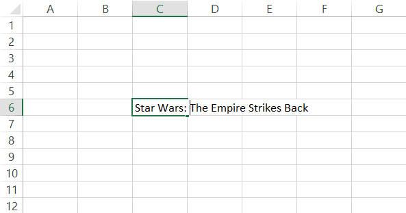
Go to C6 cell and type in ‘Star Wars: The Empire Strikes Back’. You’ll immediately notice that words will overlap onto the next empty cells to the right of C6.
Step 3: Highlight the cell you want to wrap text.
Once you’ve populated the cell or have a cell that already has a lot of texts in it, it’s time to select it for formatting. You can do this by left-clicking on the cell block that you want to text wrap. A clear indicator, such as a green border around the cell, will show when you’ve successfully highlighted the cell block.

Step 4: Click on the Wrap Text function.
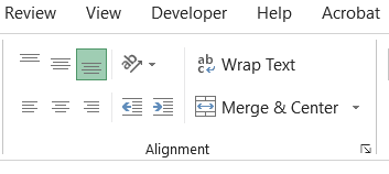
While you’ve highlighted the cell, move your mouse to the top-left corner of the Excel window. Look for the ‘Wrap Text’ button and simply left-click that feature to enable text wrapping for the specific cell that you’ve highlighted.

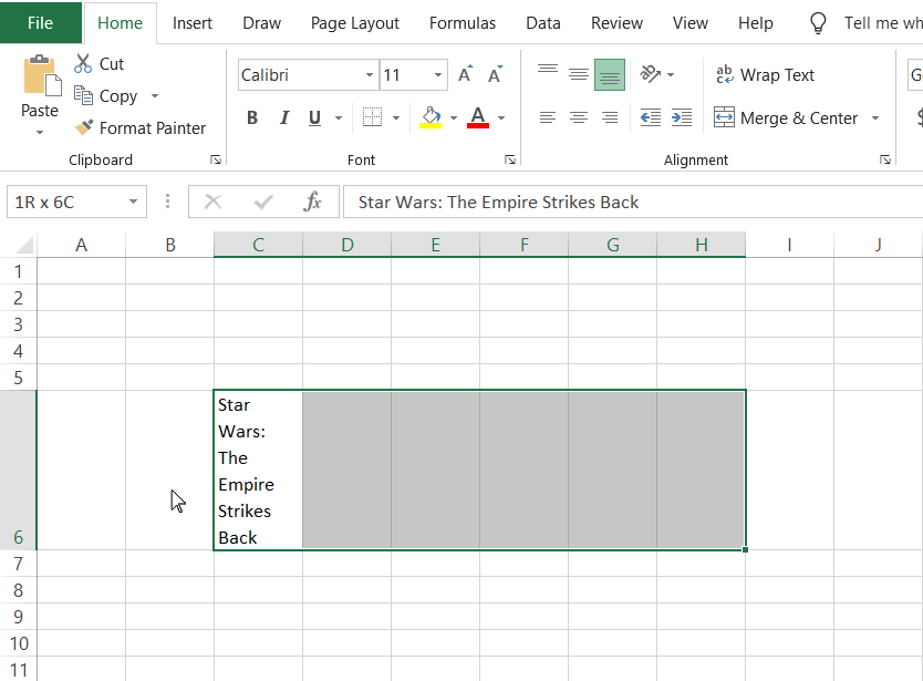
The highlighted cell should now look like this.

Congratulations! You’ve successfully wrapped the text of the cell block that was overlapping other cells. Now, here’s how you can do this process with multiple cells.
Step 5: Select and highlight multiple cell blocks.
The secret to formatting a lot of cell blocks at once is to select multiple cells at the same time. This way, any formatting or features applied will affect all the cell blocks. You can do this in two ways:
- Hold down the left-click on a particular cell block and drag it across the spreadsheet.

- Click on a cell and press Shift while moving with the arrow keys on your keyboard. You can also press Ctrl + Shift simultaneously while pressing on the arrow keys to move to highlight an entire row or column.

Once you’ve highlighted all the necessary cells, you can go ahead and click on the Wrap Text button at the top-left corner of your screen. This will apply the wrap text feature to all the cells you’ve just highlighted!
Method 2: Doing A Manual Line Break
The next method you can do is to use line breaks to wrap text. This method is suitable if you want to control the specific position where the new line should start. Unlike the automatic wrap text as shown in the previous method, this method lets you precisely adjust the line break.
Let’s go over the steps on how you can do this.
Step 1: Open up your Excel file.

Step 2: Highlight the cell you want to format.
With your Excel document open, double click on the cell you want to wrap text. We will use the same example as was used in Method 1. Go to Cell C6 and type in ‘Star Wars: The Empire Strikes Back’. You should see that the words will overlap onto the next empty cells to the right of C6.
Step 3: Place cursor at the location of the line break.
To insert a line break, place your cursor at the position where you would like the line to break. We will choose to do this after the colon ‘:’ used in the text.

Step 4: Press Alt + Enter keys.
Finally, press the Alt and Enter keys together to add the line break. As a result, you should see the line break occur with the terms ‘Star Wars:’ and ‘The Empire Strikes Back’ in different lines.

It’s worth noting that inserting a manual line break does automatically trigger the Wrap Text option in the menu. This is not a cause for worry as you still maintain your manual line break. However, the key difference is that the formatting will stay in place even if you decide to make the column wider.
Conclusion
Now that you’ve reached the end of this article, hopefully, we’ve helped you figure out how to wrap text in Excel.