Checking for the highest or lowest value in a data set comes in handy on many occasions. To do this on Google Sheets, there are easy and efficient custom formulae that you can use.
- Need to highlight the highest value within a cell range?
- Need to highlight the top three cells with the highest values?
- Need to highlight values within a single row?
We have got you covered. We have compiled the most comprehensive tutorial to guide you.
5 Methods of highlighting the highest and lowest:
Method 1: Highlighting the highest and lowest values within a cell range
1.1 Highest value within a range
1.2 Lowest value within a range
Method 2: Highlighting the highest and lowest values within a column
2.1 Highest value within a column
2.2 Lowest value within a column
Method 3: Highlighting the highest and lowest values within a row
3.1 Highest value within a row
3.2 Lowest value within a row
Method 4: Highlighting N cells with highest and lowest values
4.1 Highlight top N cells with the highest value
4.2 Highlight top N cells with the lowest value
Method 5: Highlighting the entire row with the highest and lowest values
5.1 Highlight row with the highest value
5.2 Highlight row with the lowest value
Let’s go over the methods one by one, starting with highlighting values within a cell range.
Method 1: Highlighting the highest and lowest values within a cell range
1.1 Highest value within a range
To highlight the highest value within a cell range, adopt the following steps.
Step 1: Select your range.
Select the range of cells in a column where you want the highest value by right-clicking and selecting cells or by pressing Shift and selecting the first cell and the last cell of the range. Here we are selecting cell A2:C9.
Step 2: Applying Conditional formatting.
Click on Format on the main tab. Click and select Conditional formatting from the drop-down.


A tab on the right side of your window will open up. The default option is Is not empty.
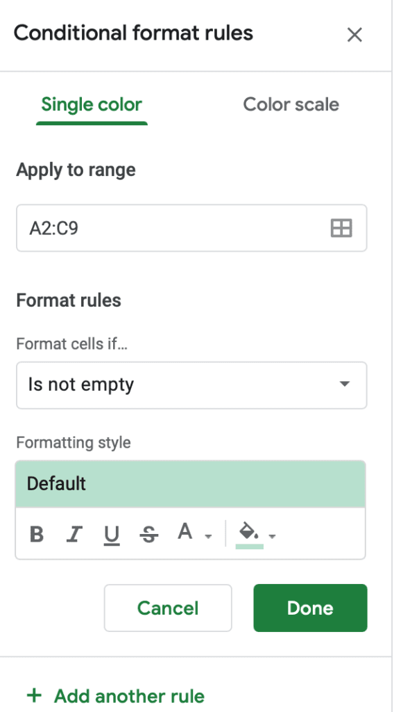
Select Custom formula is from the drop-down and add the formula with the given syntax.

Step 3: Applying the formula as per given syntax.
In the Custom formula is box add the formula according to the given syntax
= A2:A9=MAX($A$2:$C$9)

Here, the Apply to range refers to the range of cells where you apply the conditional formatting.
Click on Done to apply the formatting.
You will see the highest value highlighted in the default color, green.

If you want to change the color, simply click on the color fill option on the tab on the right side and select another from the palette that opens up.

1.2 Lowest value within a range
Follow Steps 1 and 2, given above.
Step 3: Applying the formula as per given syntax.
In the Custom formula is box add the formula according to the given syntax = A2:A9=MIN($A$2:$C$9).

Here, the Apply to range refers to the range of cells where you apply the conditional formatting.
Click on Done to apply the formatting.
You will see the highest value highlighted in the default color, green.

If you want to change the color, simply click on the color fill option on the tab on the right side and select another from the palette that opens up.
Method 2: Highlighting the highest and lowest values within a column
2.1 Highlight highest value within a column
To highlight the highest value within a column, adopt the following steps.
Step 1: Selecting your range.
Select the range of cells in a column where you want the highest value by right clicking and selecting cells or by pressing Shift and selecting the first cell and the last cell of the range.

Step 2: Applying Conditional formatting.
Click on Format on the main tab. Click and select Conditional formatting from the drop-down.


A tab on the right side of your window will open up.

The default option is Is not empty. Select Custom formula is from the drop-down and add the formula with the given syntax.

Step 3: Applying the formula as per given syntax.
In the Custom formula is box add the formula according to the given syntax = $A:$A=max(A:A).

Also, insert the range to which you want to apply the formatting in the Apply to range field. Click on the color fill tool to select a custom color instead of the default option. Click on Done to apply the formatting You will be able to see the highest value highlighted in the default color, green.

2.2 Highlight Lowest value within a column
To highlight the lowest value within a column, follow Steps 1 and 2 as outlined before.
Step 3: Applying the formula as per given syntax.
In the Custom formula is box add the formula according to the given syntax = $A:$A=min(A:A)

Click on Done to apply the formatting.
You will be able to see the highest value highlighted in the default color, green. We have selected red in the color palette for the lowest value, hence it is showing up highlighted in red.

Both conditional format rules that have been applied are now visible.
Method 3: Highlighting the highest and lowest values within a row
3.1 Highest value within a row
To highlight the highest value within a row, adopt the following steps.
Step 1: Selecting your range.
Select the range of cells in a row where you want the highest value by right clicking and selecting cells or by pressing Shift and selecting the first cell and the last cell of the range.

We have taken Row2, that is A2:C2.
Step 2: Applying Conditional formatting.
Click on Format on the main tab. Click and select Conditional formatting from the drop-down.


A tab on the right side of your window will open up.

The default option is Is not empty.
Select Custom formula is from the drop-down and add the formula with the given syntax.

Step 3: Applying the formula as per given syntax.
In the Custom formula is box add the formula according to the given syntax =A2:C2=MAX($A2:C2).

A2:C2 is the row where we are selecting the highest value.
Click on Done to apply the formatting.
You will be able to see the highest value highlighted in the default color, green.

If you want to change the color, simply click on the color fill option and select another from the palette that opens up.
3.2 Lowest value within a row
To highlight the lowest value within a row, follow Steps 1 and 2 as outlined before.
A tab on the right side of your window will open up.
Since we have applied a rule before, it will look like the screenshot given below. Click on Add another rule.

If you have not applied any other rule, you’ll have to simply select Custom formula is and apply Step 3 as outlined below.
Step 3: Applying the formula as per given syntax.
In the Custom formula is box add the formula according to the given syntax =A2:C2=MIN($A2:C2).

A2:C2 is the row where we are selecting the lowest value.
Click on Done to apply the formatting.
You will be able to see the lowest value highlighted in the color red, which we have selected.

Here you can see both the formulae that we have applied.
Method 4: Highlighting N cells with highest and lowest values
We will be highlighting a predefined number of cells that have the highest or lowest value. For selecting the range and navigating to Conditional formatting, please follow Steps 1 and 2 as outlined before.
4.1 Highlight top N cells with highest value
Step 1: Selecting your range.
Select the range of cells in a column where you want the highest value by right clicking and selecting cells or by pressing Shift and selecting the first cell and the last cell of the range.
Here we are selecting cell A2:A9 to get the highest values.
Step 2: Applying Conditional formatting.
Click on Format on the main tab. Click and select Conditional formatting from the drop-down.


A tab on the right side of your window will open up. The default option is Is not empty.
Select Custom formula is from the drop-down and add the formula with the given syntax.

Step 3: Applying the formula as per given syntax.
As an example, we are taking N as 3 but you can input 5 for displaying the top 5 or otherwise. Use syntax as =$A2>=large($A$2:$A$9,3).
A2:A9 is the range fo column A where we are selecting the highest value. We will get the top three values in column A as displayed below.

4.2 Highlight top N cells with lowest value
Follow Steps 1 and 2 as outlined previously.
As an example, we are taking N as 3 but you can input 5 for displaying the top 5 or otherwise. Use syntax as =$A2<=small($A$2:$A$9,3)
Here, A2:A9 is the cell range on which we are applying our criteria. We will get the lowest three values in column A as displayed below.

Method 5: Highlighting the entire row with the highest and lowest values
5.1 Highlight row with highest value
Step 1: Selecting your range.
Select the range of cells in a column where you want the highest value by right-clicking and selecting cells or by pressing Shift and selecting the first cell and the last cell of the range.
Here we are selecting cell A2:C9 to get the highest values.

Step 2: Applying Conditional formatting.
Click on Format on the main tab. Click and select Conditional formatting from the drop-down.


A tab on the right side of your window will open up. The default option is Is not empty.

Select Custom formula is from the drop-down and add the formula with the given syntax.

Step 3: Applying the formula as per given syntax.
As an example, we are taking N as 3 but you can input 5 for displaying the top 5 or otherwise. Use syntax as =$A2>=large($A$2:$A$9,3)
Note that A2:C9 is the range within which the row gets highlighted. The rows that are highlighted are dependent on the value of column A.
We will get the top three rows highlighted as below. The entire three rows including the values get highlighted.

To get values within column B, determine the top three rows, modify syntax as follows:
=$B2>=large($B$2:$B$9,3)

5.2 Highlight row with lowest value
Follow Steps 1 and 2 as before.
Step 3: Applying the formula as per given syntax.
As an example, we are taking N as 3 but you can input 5 for displaying the top 5 or otherwise. Use syntax as =$A2<=small($A$2:$A$9,3).
Click on Done.

You will get the lowest values from column A as given below. The entire three rows including the values get highlighted.

To make this dependent on another column’s values modify the syntax as follows:
=$B2<=small($B$2:$A$9,3)

Conclusion
Hope these methods cover all your queries regarding highlighting the highest and lowest values on Google Sheets. Drop comments for further questions and discover other helpful articles on our website.